Posts

Using Airplane Transponder Data to Characterize Antenna Performance

Image
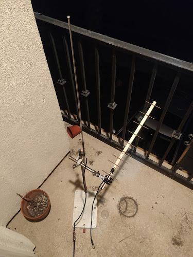
Hi All, Recently I obtained some low-noise amplifiers in order to better receive NOAA GOES satellites. A low-noise amplifier however is no good without a decent antenna. Most often people use these 2.4 GHz wifi antennas modified to operate at the GOES downlink frequency. This typically gives very good results but it's pretty challenging to DIY a satellite dish. An alternative to satellite dish type antennas is the highly directional yagi-uda antenna. Yagi-uda antennas are pretty (seemingly) simple to build so one night I made a first pass at throwing one together. Alas the satellite signal still did not appear (probably due to my poor assembly). Instead of scrapping the inadequate antenna I decided to try and figure out if adding the passive elements actually did anything to the directionality of the yagi-uda antenna versus a regular dipole antenna. To do this without some sort of signal source is typically impossible and so people resort to modelling programs that calculate the ga

SHO Perturbations with Creation and Anihillation Operators

Image
Hello, In the last post I demonstrated how to compute a perturbation on the harmonic oscillator up to fourth order. In this post we'll do the same thing but using creation and annihilation operators. The eigenvalues obtained with this method are based on diagonalizing an n by n matrix where n is the number of solutions. Since there are an infinite number of solutions the eigenvalues will converge to the true values as the dimension of the matrix increases to infinity. Since we're not going to be diagonalizing the infinite matrix we can only obtain approximate solutions to the perturbed hamiltonian. A really great resource for this and more examples/examinations of the method can be found here The creation operator takes the form: The annihilation operator is defined as: We generated the above matrices with the following code: We can then redefine the x operator in terms of our new operators, and use those to form a matrix that represents ou

Perturbation Theory in Mathematica

Hello, I've wanted to implement perturbation theory in mathematica for some time now. Here, I've done so for a non-degenerate time independent case. Specifically for the one dimensional harmonic oscillator (not quantum because symbolic constants just make the computation take longer). I tested it on some problems from Shankar's quantum mechanics book and it works. The things you'll need are: 1. Eigenvalues and eigenfunctions for a solved case (in our case the harmonic oscillator). $$H0=\frac{\text{$\#$1} x^2}{2}-\frac{\nabla _{\{x\}}^{}\text{$\#$1}}{2}\&$$ \[ScriptCapitalH]0 = -(1/2) Laplacian[#1,{x}] + 1/2 (x^2) #1 &; \[ScriptCapitalH]1 = x^2 #1 &; \[ScriptCapitalH] = \[ScriptCapitalH]0[#1] + \[ScriptCapitalH]1[#1] &; {eigList, wfnList} = DEigensystem[\[ScriptCapitalH]0[u[x]],u[x],{x}\[Element] FullRegion[1], nmax, Method -> "Normalize"]; where nmax is the maximum number of eigenvalues/eigenfunctions to compute.

Tracking Local Airplanes with an SDR and dump1090

Image
Hi, I spent the last day or so collecting data and visualizing it with Mathematica. The data was collected using a nooelec SDR and the open source software dump1090. I had initially thought this wasn't possible because this particular model of SDR has a dead spot near 1090 MHz where the signal is received. Nonetheless, the SDR is capable of receiving aircraft transponder data when fitted with a pcb digital antenna. Since San Diego is home to several airports I expected a lot of commercial air traffic, however to my surprise I was able to receive signals all the way up from Palm Springs. Over the course of the collection period I accumulated ~139 MB of data. Before we get to how I visualized the results lets look at the software and methods utilized to collect the data: dump1090 can be found here: https://github.com/antirez/dump1090 by executing $ ./dump1090 --aggressive --interactive --net --net-http-port 10900 --net-sbs-port 30003 we start a server that gives

RTL-SDR NOAA Satelite Update

Image
So the last time I wrote about my adventures into the world of software defined radio satellite reception I was dealing with some local FM radio stations really messing with my radio's ability to get a clear sat signal. This proved to be a difficult challenge to overcome as the same interference would be present, and sometimes stronger even if I went to the roof of a building to take the measurement. Nevertheless I got some nice images which are in prior posts. One of the advantages of software defined radio is that the data is read through a computer and so the radio can be made easily accessible by connecting it to a server. Many hobbyists have set up publicly accessible radios by doing this and some of them are very good resources for those living in areas with poor reception or lots of interference. You can find many of these at http://websdr.org . One radio in particular, http://k3fef.com:8902/  is equipped with a quadrifilar helicoidal antenna much like my own and is sc

Fitting TOCSY (2D 1H NMR) Data with Mathematica

Image
So this isn't so much "fitting" as it is programming in known data points and then making a function that easily allows one to switch between different inputs until one that is close enough is identified visually. It could be substantially improved by adding peak detection and error calculations. For one of my classes, Ch 007, my lab partner and I used solid phase synthesis techniques to make a pentapeptide incorporating four known peptides (one of which is non canonical) and an unknown mystery peptide in a known order. Solid phase techniques are generally known for their extremely high yields. Given that it was my first go at the technique I think I might have played a key role in obtaining a much lower than expected yield. Nevertheless, the product was purified by prep HPLC and the result was rather pure in the 1H NMR spectrum. We obtained a TOCSY 2D spectrum and are now tasked with interpreting the TOCSY spectrum as well as ESI-MS and MALDI-MS to verify the structur

Modelling a Magnetic Cube: Dipoles!

Image
So I found this paper    https://doi.org/10.1063/1.4941750  (It's open access by the way) and in it they have a nice equation for the energy between two magnetic dipoles. $$E_{m_{1}m_{2}} = \frac{1}{4\pi\mu}\frac{m_{1}m_{2}-3(m_{1}e_{r})(m_{2}e_{r})}{|l^{3}|}$$ In it, the terms m1 and m2 describe the dipole vector of each magnet, and er describes the normal vector between the centers of each dipole, l describes the distance between the two dipoles, and mu is the permeability of the medium. For our purposes I got rid of mu because it's just a scaling factor. With dipoles the determination of the energy becomes a little more complicated because I've got to permute through all the possible orientations of the magnets in order to find the best choice for moving to a lower energy. This is simplified greatly by the fact that the magnets in this case are cubes and so can only have six possible orientations. In the code I've described this with an integer (1 to 6