Modelling a Magnetic Cube: Dipoles!
So I found this paper https://doi.org/10.1063/1.4941750 (It's open access by the way) and in it they have a nice equation for the energy between two magnetic dipoles.
$$E_{m_{1}m_{2}} = \frac{1}{4\pi\mu}\frac{m_{1}m_{2}-3(m_{1}e_{r})(m_{2}e_{r})}{|l^{3}|}$$
In it, the terms m1 and m2 describe the dipole vector of each magnet, and er describes the normal vector between the centers of each dipole, l describes the distance between the two dipoles, and mu is the permeability of the medium. For our purposes I got rid of mu because it's just a scaling factor.With dipoles the determination of the energy becomes a little more complicated because I've got to permute through all the possible orientations of the magnets in order to find the best choice for moving to a lower energy. This is simplified greatly by the fact that the magnets in this case are cubes and so can only have six possible orientations.
In the code I've described this with an integer (1 to 6) which is interpreted through a set of rules which produce the vectors for the calculation of energy and for the generation of a graphical plot. This isn't strictly necessary but arose as an artifact of how I wen't about writing the program.
If you read the paper it would be clear that I'm not actually doing what they did in the paper. I'm not interested in simulating the behavior of magnets, but just in finding the lowest energy state and since I already kind of know the answer it shouldnt be too hard to make a better energy function but for now I'm just going to stick with that first equation.
Other than the new energy function I've also come up with a much more efficient way to compute the ground state configuration. As we've discussed previously, with six different possible orientations of a dipole in a cubic geometry there are 6^512 different assembled 8x8x8 cubes. Up until this point the strategy has been to start at one of these asssemblies and then optimize the orientation of each dipole until no lower energy state can be found. While this is alright for a low dimensional problem, as in the monopole square assemblies, it is substantially more challenging to find the right parameters to arrive at the ground state of a cubic assembly of dipoles. This is due in part to the large number of degenerate states. I suggest that this strategy's primary failing is that every time it makes an "incorrect" but allowed change ie switching a dipole's orientation such that there is no energy change but not moving it closer to the ground state, it has to go over every single dipole at least once in order to corect such a change. In this way, the function that describes the number of changes until the ground state is not effectively minimized by the strategy and so it is possible that the entire state space will be searched before finding the ground state. Obviously not the best route to solve the problem.
Instead, I've come up with an alternative solution, while there are 6^512 possible assembled configuration, there are only 6*512 distinct dipoles that are needed to guarantee that the ground state can be reached. That is to say that with 6*512 dipoles I can create the entire state space. That's a manageable ammount of information to work with. So if I create a list of all of these distinct dipoles, described by a three dimensional spatial coordinate system and a vector describing the orientation of the dipole I should be able to randomly select a dipole and then use the energy function to compute the energy that results from adding one of the remaining dipoles to the first choice. Then by simply taking the addition that results in the most energy loss I will compute the ground state configuration. Of course each time I "choose" a dipole from the list of possibilities we eliminate all six of the orientations from the list so that no spatial position is occupied by more than one dipole.
There is still a tiny problem with the energy function from the paper. Namely that it doesn't accurately describe the energy of the possible orientations of two magnetic cubes. Consider two cubes, one oriented along +z and the other oriented along +y, the energy equation would say that this configuration has no net energy change because the dipoles are orthogonal so the dot products go to 0. The issue with this is that the magnetic cubes are in fact destabilized in this orientation. This problem doesn't prevent us from reaching a solution though so I'm just going to ignore it for now.
Now for the program.
northCube [x_, y_, z_, dir_] :=
GeometricTransformation[{{Red,
Cuboid[{-1/2 + x, -1/2 + y, 0 + z}, {1/2 + x, 1/2 + y,
1/2 + z}]}, {Blue,
Cuboid[{-1/2 + x, -1/2 + y, -1/2 + z}, {1/2 + x, 1/2 + y,
0 + z}]}}, dir /. directionRules[x, y, z]];
directionRules[x_, y_,
z_] := {1 -> RotationTransform[Pi, {0, 0, 1}, {x, y, z}],
2 -> RotationTransform[-Pi, {1, 0, 0}, {x, y, z}],
3 -> RotationTransform[Pi/2, {1, 0, 0}, {x, y, z}],
4 -> RotationTransform[-Pi/2, {1, 0, 0}, {x, y, z}],
5 -> RotationTransform[Pi/2, {0, 1, 0}, {x, y, z}],
6 -> RotationTransform[-Pi/2, {0, 1, 0}, {x, y, z}]};
vectorRules = {1 -> {0, 0, 1}, 2 -> {0, 0, -1}, 3 -> {0, 1, 0},
4 -> {0, -1, 0}, 5 -> {-1, 0, 0}, 6 -> {1, 0, 0}};
\[Mu] = 1;
northCube is a function that generates the propper Graphics3D primitive for plotting, it accepts x, y, and z spatial coordinates and an integer value dir that describes one of six orientations given by directionRules.
e[term_, matrix_] :=
N[((term[[4]] /. vectorRules).(#[[4]] /. vectorRules) -
3 (Dot[(term[[4]] /. vectorRules),
Normalize[
term[[{1, 2, 3}]] - #[[{1, 2, 3}]]]]) (Dot[(#[[4]] /.
vectorRules),
Normalize[term[[{1, 2, 3}]] - #[[{1, 2, 3}]]]]))/(4*\[Mu]*
Pi*(EuclideanDistance[
term[[{1, 2, 3}]], #[[{1, 2, 3}]]])^3) & /@ matrix]
e is the energy function that accepts a dipole term and a matrix of dipole terms and computes the energy between the term and every element in the matrix. Note that this version of the energy function does not sanitize the matrix of term because the sanitization is done in the computation of the values in matrix.
dim = 3;
allConfigs = (*Cube*)
Flatten[Table[Append[#, n] & /@ Tuples[Range[dim], 3], {n, 1, 6}],
1];
allConfigs1 = (*Square*)
Flatten[Table[
Flatten[Append[#, {1, n}]] & /@ Tuples[Range[dim], 2], {n, 1, 6}],
1];
growing = {};
seed = {{1, 1, 1, 1}};
AppendTo[growing, #] & /@ seed;
While[Length[growing] <= (Length[allConfigs]/6), {
newOptions =
DeleteCases[
If[#[[2]] == Length[growing], #[[1]], Null] & /@
Tally[Flatten[
Delete[allConfigs,
Position[#[[{1, 2, 3}]] & /@
allConfigs, #[[{1, 2, 3}]]]] & /@ growing, 1]], Null];
If[Length[newOptions] == 0, Break[]];
eList1 = Total[ e[#, newOptions] & /@ growing];
eList = e[Last[growing], newOptions];
growing =
AppendTo[growing,
Flatten[newOptions[[
Flatten[RandomChoice[Position[eList, Min[eList]]]]]]]];
}]
dim is the number of terms along one side of a cube or square, allConfigs describe either the possible terms of a cube or square with side length dim. Growing is a list used to store the growing matrix, seed is the first term, which can also be randomly selected. The while loop uses a condition that computes the expected number of elements in the completed assembly and stops once this value is reached. Or rather it compares 1/6 of the possible terms (the number of elements in the completed assembly) to the length of the assembly. newOptions is allConfigs with any already selected term and it's spatial equivalents deleted. Every time we select a term to add to growing, newOptions decreases by six elements. Next we make sure that there are remaining values in newOptions, if not then we break from the while loop. eList1 and eList are two different ways to compute the next move, eList1 is more computationally intensive and slows down substantially as the matrix grows but it computs the total energy of growing with every term of newOptions. eList however computes only the energy between the last element of growing and every term of newOptions, and so eList actually gets a bit faster as the computation proceeds. The lsat part of the while loop then adds the best choice from newOptions according to the eList function selected to add to growing then the whole thing repeats.
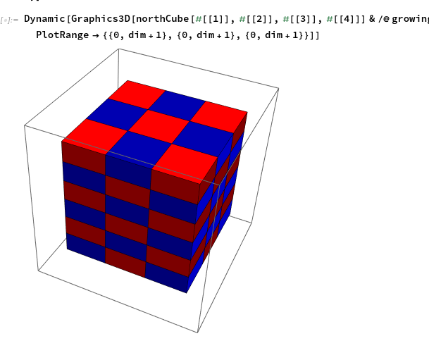
Dynamic[Graphics3D[
northCube[#[[1]], #[[2]], #[[3]], #[[4]]] & /@ growing,
PlotRange -> {{0, dim + 1}, {0, dim + 1}, {0, dim + 1}}]]
The above code is used to visualize the growing assembly.
The cool thing about this approach is that we can seed it with any possible assembly of the terms. Provided that each spatial position is only singly occupied. The advantage of this is that I can rapidly compute the ground state configuration of an 8x8 square using eList1. To do so with an 8x8x8 cube however is very sluggish and leads to offtarget results. However using this 8x8 squre as the seed I can generate the ground state configuration of the 8x8x8 cube using eList and so arrive at a solution rapidly. Because the square seed begins each column of the cube with the correct orientation, off target results are entirely avoided because the addition of an orthogonal dipole is always second best to the addition of a dipole in the same orientation.
I had a lot of fun with this project and I'm glad that I came up with a strategy that did not necessitate moving to python.
Thanks for reading,
Alex Krotz

Comments
Post a Comment