Modelling a Magnetic Cube: Monopoles

I took an interesting course this past term on biochemical computation. It's taught by Erik Winfree who was one of the first to identify that DNA strands can be used to model computation. On one of the homework assignments it was announced that the best solution would get a prize at the end of the term. Although I did not get first play, my solution was "within epsilon of winning" and so I too got a first place prize. The prize was an 8x8x8 cube of small cubes of neodymium cubic magnets. The cube was all well and good before I began dissassembling it but when the task of reassembling the cube came up I realized that although it was tauted as a "self assembling" cube, actually getting it to its most stable configuration is quite challenging. The easiest way of doing it is to make a one dimensional chain of cubes and then fold it into an 8x64 rectangle with the poles oriented parallell with the short side, then folding this rectangle into a cube. I can see why this is a readily accessible configuration (because at each step it's in a stable state), but I was inspired to try and model the configuration of a cubic set of magnets so I could compute the stability.

I decided to begin with modelling monopoles, that is, points arranged at integer positions that are either "north" or "south." A pole will interact with another like pole repulsively, destabilizing the position and increasing its energy proportional to the inverse of the euclidean distance between them. Opposite poles interact attractively and decrease the energy proportional to the inverse of the euclidean distance.

A quick note, I'm working with a 20x20x20 set of points just because it's a bit more visually interesting, the computation can easily be scaled to any size of cubes but increases substantially in time to completion.

The code is for mathematica, hopefully I'll be able to attach the notebook to this post.

Matrix generation:
matrix = Table[RandomInteger[1], {x, 1, 20, 1}, {y, 1, 20, 1}, {z, 1, 20, 1}];

Then we'll index all the positions in the matrix:
poslist[matrix_] := Table[{x, y, z}, {x, 1, Dimensions[matrix][[1]], 1}, {y, 1, Dimensions[matrix][[2]], 1}, {z, 1, Dimensions[matrix][[3]], 1}]

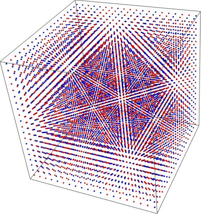
We can generate a quick plot of these with red and blue corresponding to each pole type.
Graphics3D[If[matrix[[#[[1]], #[[2]], #[[3]]]] == 1, {Red, Sphere[#, .1]}, {Blue, Sphere[#, .1]}] &/@Flatten[poslist[matrix], 2]]

Next we can make a simple hamiltonian operator which takes two positions pos1 and pos2 and generates the energy term between them. 

Ham[pos1_, pos2_] := ((matrix[[pos1[[1]], pos1[[2]], pos1[[3]]]] - matrix[[pos2[[1]], pos2[[2]], pos2[[3]]]]) /. {0 -> +1, 1 -> -1, -1 -> -1})/(EuclideanDistance[pos1, pos2]^2)

Now we'll write a function that takes a position in a given matrix and generates the energy of that position by adding up all the energies between it and the other positions in the matrix. 

e[pos_, matrix_] := N[Total[Ham[pos, #] & /@ Flatten[Delete[poslist[matrix], pos], 2]]]

Then we can generate a list of all the energies for each position in the matrix:
eList = e[#, matrix] & /@ Flatten[poslist[matrix], 2];

Before I go on to the final most illustrative plot I thought I'd include a quick aside on a visualization method using the DimensionReduce function to map the three dimensional set of points onto two dimensions, since there is no loss of information by doing this there are 1000 points each corresponding to a point in the matrix.
dimRed = DimensionReduce[Flatten[poslist[matrix], 2], 2];
I'm assuming that the order of the points is unchanged but I've yet to figure this out for sure.
ListPlot3D[Flatten[{dimRed[[#]], eList[[#]]}] & /@ Range[Length[dimRed]]]

Now for the pièce de résistance, a graphic of the points with radius corresponding to the magnitude of energy and shade corresponding to stabilization or destabilization (dark corresponds to stabilized, light corresponds to destabilized)
Graphics3D[If[matrix[[Flatten[poslist[matrix], 2][[#]][[1]], Flatten[poslist[matrix], 2][[#]][[2]], Flatten[poslist[matrix], 2][[#]][[3]]]] == 1, {Red, Sphere[Flatten[poslist[matrix], 2][[#]], If[eList[[#]] > 0, eList[[#]]/Max[eList], eList[[#]]/Abs@Min[eList], 0]]}, {Blue, Sphere[Flatten[poslist[matrix], 2][[#]], If[eList[[#]] > 0, eList[[#]]/Max[eList], eList[[#]]/Abs@Min[eList], 0]]}] & /@Range[Length[Flatten[poslist[matrix], 2]]], PlotRange -> All]

Okay I know it's not quite what I implied I would be doing in the title or intro to this post but modelling dipoles complicated it more than was necessary for me to work out the mechanics of the code. With the current code it would be pretty straightforward to write a new hamiltonian that takes the orientation of the dipoles into account.

Thanks for reading,
Alex Krotz