Modelling a Magnetic Cube: Optimizing an 8x8 grid of Monopoles

I was quite excited by the result obtained in the previous post from this series. However after acheiving it I realized that although I could propose a configuration and illustrate its energy distribution it was pretty much useless for finding what the minimum energy configuration of an arbitrary arrangement of positions each containing a monopole is.
In order to find the energetic minimum, one could in theory simply characterize the entire state space of a configuration. Since there are two possible monopoles that can occupy a position the size of the state space is 2^N for N positions. Obviously for an 8x8x8 cube that is 13,407,807,929,942,597,099,574,024,998,205,846,127,479,365,820,592,393,377,723,561,443,721,764,030,073,546,976,801,874,298,166,903,427,690,031,858,186,486,050,853,753,882,811,946,569,946,433,649,006,084,096 possible configurations. I don't think I have the resources to characterize the whole state space so we need a more efficient way of finding the energetic minimum.

For convenience I chose to work with just an 8x8 grid of positions, so 2^64 possible arrangements (still 18,446,744,073,709,551,616 arrangements) because my computer can compute the energy of a position reasonably quickly.

Instead of doing what I did in the last post and walking you through the code I'm going to just explain how it works and why it works, then paste the code at the bottom and it can be run if you've got a working install of mathematica.

I rewrote some of the functions from the last post to accept a new matrix as an input in addition to the previous input, we then generate a list of positions based on the dimensions of the matrix. These positions are used to itterate over every position in the grid. We seed the program with a grid of only 1's, a highly energetic state. As we itterate over each position, the energy of the state is computed and compared to the energy of the state if that position's value were switched (ie 1 -> 0, or 0 -> 1). If the difference in energy is less than +3.5 we accept the switch and start over with the new state.

The purpose of allowing a +3.5 increase in energy is that there are a number of local minima in the potential energy surface we are traversing. Because of this, if we restrict the acceptable switches to only those that decrease the energy, we would get trapped in a local minimum and never reach the lowest energy state.

The value +3.5 was found by trial and error and as of know I know it works for grids of dimension 5x5 to 8x8. If it is increased too much then the ground state would not be effectively trapped and the program would not terminate even if it found it.

Regarding the termination of the program, with propper setting of the energy difference parameter (+3.5 in this case), the program will not accept any further changes to the ground state and then after one more itteration over every position (+1 just to be sure) it will stop running.

Run the following code to initialize the necessary functions:
poslist[matrix_] :=
  Table[{x, y, z}, {x, 1, Dimensions[matrix][[1]], 1}, {y, 1,
    Dimensions[matrix][[2]], 1}, {z, 1, Dimensions[matrix][[3]], 1}];
Hamf[pos1_, pos2_,
  matrix_] := ((matrix[[pos1[[1]], pos1[[2]], pos1[[3]]]] -
      matrix[[pos2[[1]], pos2[[2]], pos2[[3]]]]) /. {0 -> +1,
     1 -> -1, -1 -> -1})/(EuclideanDistance[pos1, pos2]^2)
ef[pos_, matrix_] :=
 N[Total[Hamf[pos, #, matrix] & /@
    Flatten[Delete[poslist[matrix], pos], 2]]]

Then the following code is what does the minimization (dont run it yet):

t = 0;

searchData = {};

stateSpace = {};

seedMatrix = 

  Table[1, {x, 1, #[[1]], 1}, {y, 1, #[[2]], 1}, {z, 1, #[[3]], 

      1}] &@{5, 5, 1}; (*Adjust this part to change the matrix dimension*)

initPos = seedMatrix;

flatPos = Flatten[poslist[seedMatrix], 2];

pos = 1;

While[t - lastChange <= Length[flatPos],

 {oldE = Total[ef[#, seedMatrix] & /@ flatPos]; 

  randomPos = flatPos[[pos]]; 

  newMatrix = 

   ReplacePart[seedMatrix, 

    randomPos -> 

     If[seedMatrix[[randomPos[[1]], randomPos[[2]], 

        randomPos[[3]]]] == 1, 0, 1]]; 

  AppendTo[stateSpace, { t, Total[neweList]}];

  neweList = ef[#, newMatrix] & /@ flatPos; 

  If[(Total[neweList] - oldE) <= (*for 8x8x1 and 5x5x1 3.5*)

    3.5, {lastChange = t, seedMatrix = newMatrix, 

    AppendTo[searchData, Total[neweList]]}]; t = t + 1;

  If[pos < Length[flatPos], pos = pos + 1, pos = 1];

  }]

Before running the above code though make sure to run: 

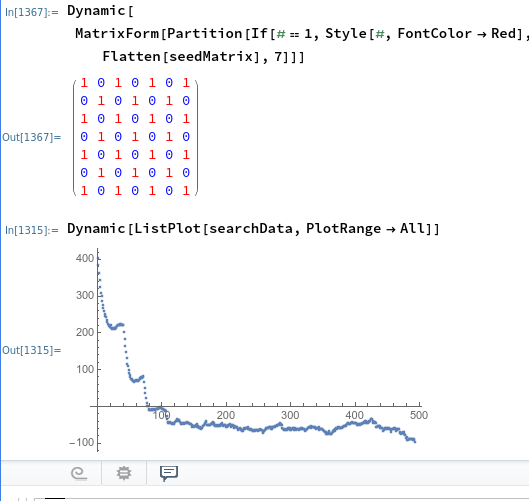
Dynamic[MatrixForm[

  Partition[

   If[# == 1, Style[#, FontColor -> Red], 

      Style[#, FontColor -> Blue]] & /@ Flatten[seedMatrix], 5(*change this number to the dimension*)]]]

to view the dynamically updating grid

and the following to show the energy path it is taking. 

Dynamic[ListPlot[searchData, PlotRange -> All]]

I tried optimizing a 9x9x1 grid but it took waaaaaay too long. Here's a screenshot of the 7x7

I'm going to try and get a screen capture video of it running so you can see it in realtime, but running the code works pretty well. 

Here's a good example of what happens when the loss parameter is set too high. The repeating pattern that the program get stuck in is indicative of this. 

When the parameter is just right, 3.2 in this case, the ground state can be found quite rapidly. 

Thanks for reading,

Alex Krotz